Optimal design of a greenhouse cooler with a cross-flow fan.

Abstract

Here I give the procedure to arrive to optimally couple the number of countercurrent theoretical units of a fine wire heat exchanger to the parameters of a cross-flow fan and to the greenhouse climate. It appears that the optimal number of heat exchange units NTU = St/f · ψ/φ², where St is the Stanton number and f the Fanning friction factor characterizing the heat exchanger cloth, and ψ and φ are the optimal, that is with the maximal ψ·φ product, dimensionless pressure gain and air flow of the fan with the same opening as the heat exchanger. This fan has to be dimensioned so that NTU is around 0.6 when cooling a greenhouse which is at 30°C and 85% relative humidity. At this value the ratio ΔH/NTU is maximal, ΔH being the enthalpy difference between entrant and exit air of the heat exchanger. At that point we have the most cost-efficient heat extraction from the moist greenhouse air. From these two equations all design parameters of the heat exchanger/fan combination can be easily derived. The Fine Wire Heat exchanger cloth has an essentially higher St/f value than any other type of heat exchanger surface, even surpassing the Chilton-Colburn limit that applies to all hitherto known heat exchangers. This high heat transfer / friction ratio is in condensing mode up to 10 to 30 times higher, making greenhouse cooling, and therefore closing, an economically sound proposition. So we need fans with a ψ/φ² of about 1 in the maximum efficiency point, which is just possible with cross flow fans with forwardly curved blades.

The greenhouse

The challenge is to cool a greenhouse in summer, so that the roof can remain closed, the heat being collected in an aquifer, stored at 25°C, this heat being reused in winter and at night to heat the greenhouse so that plant growth can continue. Fuel use for heating is replaced by electricity use for the aquifer pumps and, more important, for transporting the greenhouse air by fans through the heat exchangers. Net fuel savings can reach 95 %. When the large surplus of heat at 24°C from the seasonal storage can be used outside the greenhouse, replacing fuel, and when other cycles, such as those of irrigation water into drinking water, carbon in waste into carbon dioxide and electric energy, and N, P, K nutrients from waste into irrigation for the greenhouse plants can be closed, as in "Greenhouse Village", the total net fuel savings, referred to a conventional fuel-heated greenhouse, can reach 200%. In that case we can speak of "an energy-producing greenhouse".

The climate

As a rule, the greenhouse has to be kept below 30°C, the optimal humidity is a water vapor deficit from saturation of 2 g/kg air, which translates at 30°C to 85% relative humidity and an enthalpy of 91.5 kJ/kg dry air referred to 0°C, 0% RH, 101.3 kPa. In winter, the greenhouse has to be heated to 19°C, even when it freezes outside. This heating is always possible when enough heat transfer equipment has been installed for cooling in the hot season, where insolation power can reach 650 W/m² through the roof.

The Fine Wire Heat Exchanger

With conventional heat exchangers, this 650 W/m² cooling is only economical when large amounts of cold water are flown through the coolers, so that the heat removed cannot be reused. Another method uses a heat pump, which requires a substantial amount of electric energy, the COP or ratio of heat transported / electricity used being 3 to 5. With a fine wire heat exchanger, the COP can reach 60, as we will show. The fine wire heat exchanger has the peculiar property that condensation on fine wires takes the form of a row of very fine droplets and cannot form a heat flow impeding layer, and therefore increases its heat transfer coefficient by a factor of up to 4 when condensing water vapor, which is the normal mode of operation in a cooled and closed greenhouse. To minimize airflow and thus fan power, we want to cool the air to an optimum exit temperature. When this temperature is too high, we do not condense enough water from the air to collect heat. When this temperature is too low, we condensate not much mor because the water content is too low. There is an optimum number of theoretical units, only depending on the greenhouse climate and on the water inlet temperature. To minimize investment, we cool a part of the aquifer to 8°C using a cooling tower in winter. The heat exchanger investment is determined by the maximum cooling power with the greenhouse at 30°C and 85% RH and the cooling water at 8°C, heating up to 26°C. The last number is fixed by the maximum allowed injection temperature into the aquifer. The optimum air exit temperature is now 24°C, as we shall see.

Heat exchanging cloth

The fine wire heat exchanger surface takes the form of a cloth of 100μ diameter fine copper wire connected with a large number of copper capillaries of less than 2 mm in diameter, so that even with large heat flows the water-to-copper heat transfer is not limiting the heat transfer from water to air. This requires the capillary spacing to be a few mm when large heat flows are required. The cloth is characterized by the Fanning Friction Factor f and the Stanton number St. Both can be measured in a small measurement model of the heat exchanger. They appear not to be dependent on the Reynolds number.

Cross flow fan

The fan type that matches the fine wire heat exchanger in its most compact form is the cross flow fan. This is, because the countercurrent water-to-air fine wire heat exchanger takes the form of a stack of evenly spaced mats, the width of which equal to the fan cage diameter, the stack length equal to the fan cage length, the mat spacing and length determining the NTU. The second reason is, that the low values of ψ/φ² necessary to get an optimal NTU with the values of St/f measured on the cloth, are only easily reached with drum type fans with forward curved fan blades.

Optimal design

We will now characterize the cloth, the heat exchanger and the fan in dimensionless numbers, to make the calculation more general. After that, we will put in the values that are or can be attained by cloth and fan and that are permitted in a greenhouse, and arrive at design dimensions.

The cloth

The fine wire cloth is characterized by its heat transfer as a function of air speed and condensation of water vapor, and by its momentum transfer or friction from cloth to air. Because the performance of the cloth is most important in the moment of peak insolation or peak heat flow in cooling, we concentrate on this condition that determines the investment cost in the greenhouse. The dimensionless parameter describing friction is the Fanning friction factor f, the ratio of momentum transfer or shear stress at the cloth surface to half the momentum convection or Bernoulli term ½ρv² of the air flow, v being the empty channel air speed. The pressure drop over the heat exchanger with friction [or heat transfer] surface A and frontal surface A_c then becomes: Δp = A/A_c · f · ½ ρ v². Experiments have shown that in the practical [turbulent] range of operation, f does not much vary with the Reynolds number. The dimensionless parameter describing heat transfer is the Stanton Number, St = α / [C_p · ρ · v], the ratio between transferred and convected heat. Experiments have shown that in the practical [turbulent] range of operation, St does not much vary with the Reynolds number and, most importantly, also not when the transferred heat is mainly latent heat, originating from diffusion of water vapor to the cloth surface with its below-dew point temperature, and condensing on the fine wires. The heat transfer coefficient α does vary; at least a factor of 10 in the operating range.

Measurements of f and St

Measurements by Marian Vlot, Masters thesis, Delft University of Technology, Department of Applied Physics, June 2003, have shown that with woven cloth we can reach f = St = 0.02, whereas in practical plate fin heat exchangers, f = 0.03 and St = 0.006. From this thesis the following two figures; the Prandtl number is just a material constant of air; Pr=0.7, Pr^2/3=0.79.

Condensation effects on heat transfer

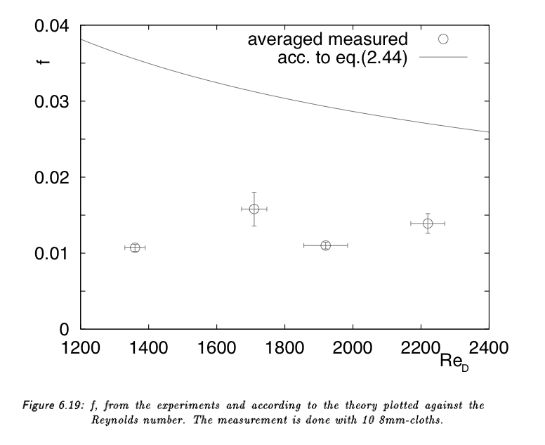
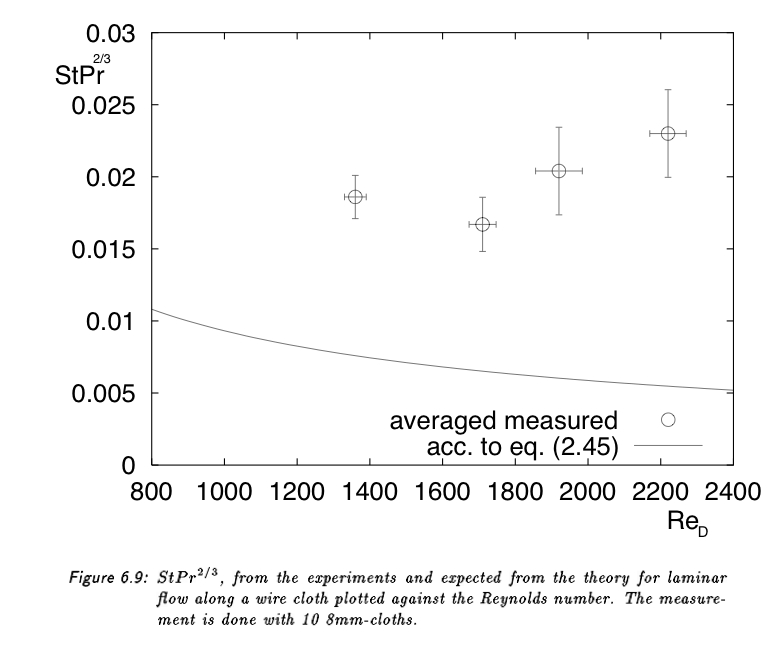
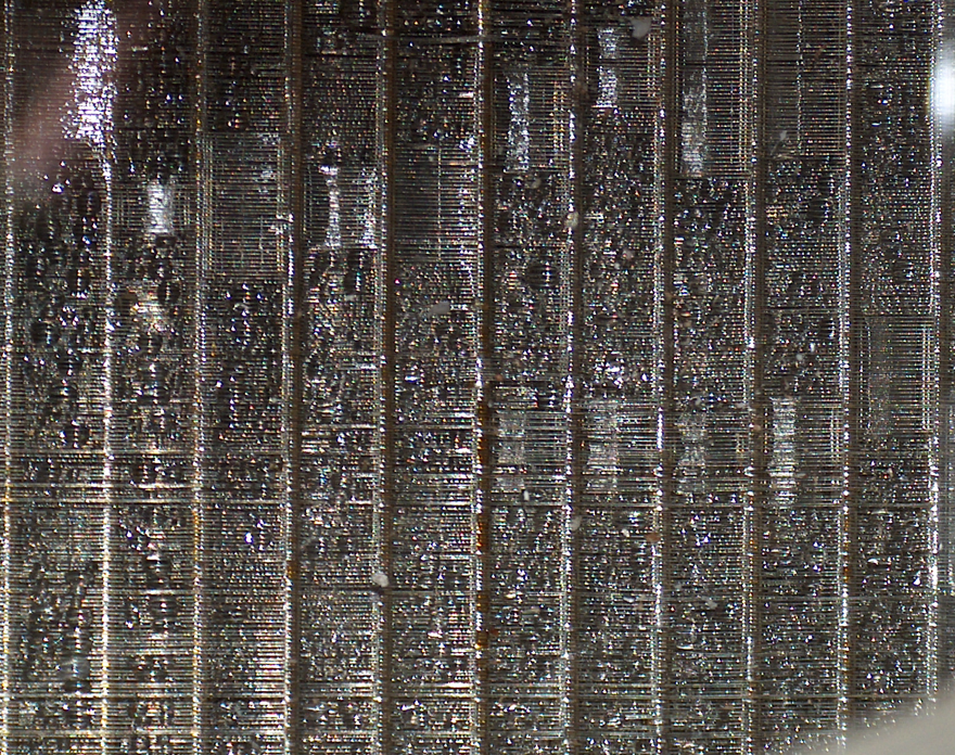
When condensation takes place, the plates are covered with a water film, causing f to rise and St to fall down. When the plates are too close to each other, the water condensed sticks between the plates and has to be blown out with certain intervals to restore the heat transfer properties. This limits the use of plate fin heat exchangers severely in the greenhouse cooling condition. With fine wires, the condensate can only take the form of very fine drops, because on a fine wire, this is the minimum energy state due to surface tension, even in the case of zero contact angles. The photograph hereunder has been taken under greenhouse cooling conditions. The result is that the Stanton number does not change when condensation takes place. The heat transfer coefficient rises substantially under condensation, because of the diffusion of water vapour from air to the wires under dew point.

The heat exchanger

The countercurrent heat exchanger is characterized by NTU, the number of "theoretical units" or heat transfer equilibrium stages. We define NTU in the air stream as 2 · [T_{air, in} - T_{air, out}] / {[ T_{air, out} - T_{water, in}] + [T_air,in - T_water,out]}, that is the ratio of air stream temperature lowering to the mean temperature difference between air and water. From the heat balance over the heat exchanger we see that α · A · {[ T_{air, out} - T_{water, in}] + [T_air,in - T_water,out]} / 2, the heat transferred, is equal to C_p · ρ · v · [T_{air, in} - T_{air, out}], the heat taken away or convected by the air. C_p here is taken to be the total heat capacity, not only the sensible part, but also the latent part due to water vapour condensation. Combining this with the definition of St, we get: NTU = A/A_c · St. We leave out small second order effects due to the fact that the latent part of Cp is not a constant along the heat exchanger, but varies with water vapor saturation pressure and therefore with temperature. It appears that under proper conditions, NTU is indeed not dependent on air speed or temperature differences, or even the amount of condensation. The last independence is due to the fact that for a gas, the equations describing the the diffusion of water vapor to the cold cloth are homologous tot those describing the momentum transfer to the cloth. The cooling power of the heat exchanger is ΔH · ρ · v · A_c, where ΔH is the difference of moist air enthalpy between air in and air out in J/kg air, as tabulated in the Mollier diagram.

The fan

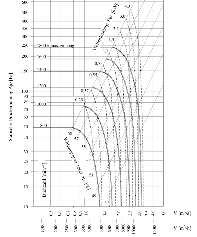
For reasons of compactness we take here a cross-flow fan. Any fan can be characterized by the dimensionless numbers ψ = Δp / [ρ · u²] and φ = Φ_v / [d · l · u], relating pressure drop Δp and volume flow Φ_v to tip rotor speed u, rotor diameter d and rotor length l. As an example, let us take the kennlinien of the LTG cross-flow fan type TW with a rotor diameter of 150mm and 1264mm length.

For instance in the point Δp_f = 240 Pa and Φ_v or V = 1.3 m³/s. This is the maximum pressure and delivery point, but also a maximum efficiency point of the fan. The rotation speed is here 1800 rpm, the rotor diameter 150 mm, rotor length 1264 mm, so u = π · 0.15 · 1800 / 60 = 14.1 m/s. Then we have ψ = 240 / [0.5 · 1.2 · 14.1²] = 2.01 and φ = 1.3 / [0.15 · 1.264 · 14.1] = 0.155. Further inspection shows that for other rotation speeds, ψ and φ in the max. efficiency point do not vary. In fact, they are determined by fan and housing design, rather than by rotating speed.

The optimal design of the heat exchanger

Now, given the values of ψ and φ along the fan curves and f and St of the cloth, we have to design the optimal A, A_c and NTU of the heat exchanger. First, it makes sense to make A_c = d · l, for reasons of compactness. So in the case of the LTG fan, we make the cloth pieces 150 mm wide, cut them on a length and stack them with a spacing to be optimized to have a heat exchanger 1264 mm long. In this case, Φ_v= v . A_c and after elimination of u, v and Δp we get the simple formula Nu = [St/f ] · ψ/φ². This applies for any cloth and any fan provided that the cloth width is equal to the fan diameter. It means that the heat exchanger air impedance is fitted to the fan air impedance, so that the fan, regardless of rotation speed, is always working in its maximum efficiency point. We also get A/A_c · f = ψ/φ², and these two dimensionless equations give us all the dimensions that we need. But, as ψ/φ² varies from zero to infinity along the fan curve, we need also to know where on this curve we have the most cooling power. To this end we tabulate a number of different air exit temperatures, and the enthalpy of air at these temperatures at water saturation point, which we can look up in the Mollier diagram on the saturation line. The enthalpy of the greenhouse air at 30 °C and 85% relative humidity is 91.5 kJ/kg, so that we can now calculate ΔH-air. With the same air exit temperature we can calculate NTU = 2 · [T_{air, in} - T_{air, out}] / {[ T_{air, out} ­ T_{water, in}] + [_Tair,in ­ T_water,out]}, we take here the cooling water entering at 8°C and exiting at 26°C.
Now to arrive at optimal cost/performance, we define the heat exchanger cost as proportional to the cloth surface and the fan cost, including the present value of its electricity use over the investment horizon, as proportional to the air power: fwx-cost = CH·A and fan-cost = CF ·Δp · Φv where the air volume flow Φv = v · A_c. The total cost now becomes CH · A + CF · Δp · Φ _v· A_c. The performance is the cooling power or ΔH-air · ρ · v · A_c at the conditions that determine the investment. We have 2 parameters to optimize: The A/A_c of the heat exchanger and the air speed v. The cost/performance is (CH · A + CF · ρp · v · A_c) / ΔH-air · ρ · v · A_c, and by separating the two parameters to optimize, and remembering that Δp = A/A_c · f · ½ ρv² we can write A/A_c/ρ/ΔH · (CH/v + CF · f · 0.5 · v²). Now the minimum value of the last factor is 3/2 · CH^2/3 · CF^1/3 · f ^1/3 at the optimal v = (CH/CF/f/ρ)^1/3 = 7.45 m/s when we take as an example CH = 200 €/m² cloth [double] surface and CF = 20 €/Watt air power. Now we have to find the minimum value of A/A_c/ρ/ΔH, and remembering that NTU = A/A_c · St we just have to find the minimum of NTU/ΔH. Quite independent of variables other than the greenhouse climate, we find that an air exit temperature of 24 °C yields the minimum value of NTU/ΔH = 0.0321 kg/kJ at NTU = 0.6.

This value gives us the optimal cloth surface of 30 times the fan or heat exchanger opening A_c, or an optimal pressure drop of 20 Pa and an airflow of 7.45·0.15·1.264·3600 = 5085 m³/hour. Putting the last two values in the fan kennlinie we see that we arrive at 870 rpm, a suboptimal efficiency of 51%, and a fan electric power of 0.37 kW. The cooling power is 26.8 kW, so we have an energetic coefficient of performance of more than 100. We see also that the fan-heat exchanger combination will improve if the design of the fan blades and housing were changed as to give a lower ψ/φ² with the same or better electrical to air power efficiency.

Other considerations

With an air speed of 7.45 m/s, we cannot put the coolers in the greenhouse so that the air jet exiting from the fan is directed to the foliage of the plants. So we must either hang the coolers above the canopy, or position the air stream upwards between rolling tables full of plants, or provide for a suction chimney between and reaching to the top of vertically growing plants in substrate gutters and direct the jet to under these gutters. We see also that the cost does not much increase using this fan, when the pressure drop increases from 20 Pa to 30 or 40. So we have the freedom to experiment with ducts to mix the greenhouse air without directing the jet to the foliage.

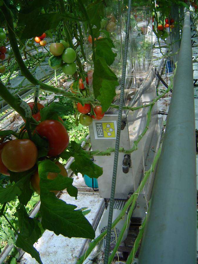
In this photo we see a fine wire heat exchanger following this optimal design procedure, lodged one per 40 m² greenhouse floor between the tomato plants of "De Groene Tuin" BV in Berlicum, Friesland, The Netherlands, cooling maximally 25 kW, blowing the exiting air jet in horizontal direction just above the floor and below the substrate gutters in which the plants grow, and taking in its warm air just above the canopy of the culture through a highly transparent plastic foil chimney rising between the plants. This adds about 20 Pa tot the total pressure drop, but the design stays quite near optimal. The mixing time of the greenhouse air is a few minutes, so the climate is homogeneous. The gentle air flow between the plants, about 1 m/s, enhances water vapor transport from and CO₂ to the leaves, stimulating growth. This experiment was made possible by SenterNovem sponsoring in the EOS Demo program for saving fossil fuel in the Netherlands.